Tables were introduced in Excel 2007.

Tables are backbone of next six components of Modern Excel. Slicers, Data Model, Measures, Power Pivot, Power Query, and Power BI work only when data is in Tables.

Adopt them. Get addicted to them. You will say "why did I not know about them all these days"!

1.  With data in a Table, the Pivot Table can be used for life. Add new rows or columns. The Table expands automatically. Refresh your Pivot. The new data gets added to all the pivot reports. You will not have to readjust the data range for Pivot Table!

2.  Downloaded data runs into hundreds, if not thousands, of rows. You filter them the traditional way. You can filter data sets with thousands of rows very comfortably using Slicers. But Slicers work only when the data is in a Table!

3.  Do you want to forget “double-click” to copy your formulas? If Yes, convert data into Tables. The formulas fill up and down automatically!

4.  You do not have to keep formatting your dates and numbers “your way” when you use Tables. Formatting, including Conditional Formatting, fills up and down automatically!

1.  You cannot copy or move multiple sheets if any sheet contains a Table.

2.  Tables do not expand automatically on protected sheets, even if the cells below the table are unlocked.

3.  Custom Views are not allowed in a workbook that has one or more Tables.

4.  Rows cannot be deleted across tables within a sheet. Need to right click inside the table, then delete table specific row.

5.  Duplicate Column Headers are not allowed. Every column needs to have a unique name.

1.  Place your cursor in a cell within the data range you want to convert to Table.

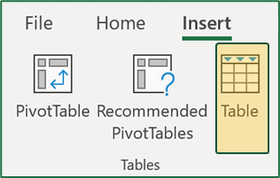
2.  Click on Insert tab. Click on Table icon.

3.  If your data has column headers, Excel Intellisense will automatically select the checkbox. If it is not ticked automatically, you need to manually select it if your data has column headers. If you are inserting Table on blank cells, let the check box remain un-selected. Excel will create a Column Header row automatically.

1.  Keep cursor in a cell that has data. Use CTRL + T keys to insert Table. The “My table has headers” button must be checked if your data already has column headings.

2.  Use CTRL + L while working in Excel Online. CTRL + T add a new Tab in the web browser!.

1.  Freeze Rows with your cursor below the “Headings” row of tables. This will ensure visibility of column names (A, B, C....) while scrolling down.

2.  Name the Table. Ideally, start the Table name with Tbl. To name a Table, click on "Table Design" ribbon. First group (Properties) has a text box to type table name. Please remember that spaces are not allowed in table name.

3.  Insert 5-6 rows above the Column Title row. These can be used for Slicers, Notes, Formulas, etc.

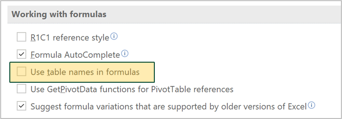
1.  This is default setting. In the initial few months, it is better to switch off column names and use cell reference in the formulas.

2.  To change default settings: File >> Options >> Formulas >> Working with Formulas. Un-tick “Use table names in formulas"

There can be two reasons:

1.  When we type any data in a cell, it is not automatically copied across all rows. Thus, the automatic Formula Fill gets disabled. To solve,

  a.  Delete all the data in the column. Type a formula. It should autofill.

  b.  If challenge persists, delete the column and insert new column!

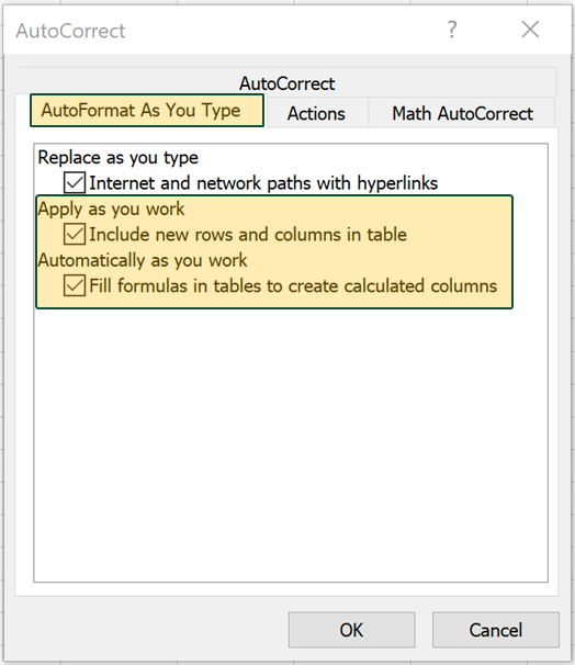
2.  The default settings have been altered. Change them.

     File >> Options >> Proofing >> AutoCorrect Options >>“AutoFormat as You Type” tab. “Include new rows....” and “Fill formulas in tables....” should be selected.

To see list of all tables in your workbook:

Formulas tab >> Name Manager

We can use these rows for:

1.  Slicers: Increase height of row 1 to 100. This creates horizontal space for slicers, without over-lapping table.

2.  Formulas: =COLUMN() function to get column number, =SUBTOTAL() for COUNT and SUM of all rows (even after filtering).

3.  For ABSOLUTE reference data like, Dates (in budgets), Commission / Interest Rates, Currency Exchange Rates, etc.

4.  For MERGE and CENTER cells of columns pertaining to same measure. Like FY in Budgeting, Region in Sales Analysis, etc.